Tip of the Week: How to Freeze Excel Rows and Columns

Modern office workers spend lots of time entering data and crunching numbers with Microsoft Excel. Therefore, it’s essential that Excel users know how to best navigate a spreadsheet. One of the best ways to make Excel easier to use is by freezing its rows and columns.

It may be a pain point for Excel users to view a spreadsheet that’s larger than their screen. It can be annoying to try and scroll up, down, or sideways, only to have a crucial piece of information that you want to reference scroll off screen. The best way to prevent this is to freeze a needed row or column into place so that it doesn’t move while you scroll through your spreadsheet. Here’s how you do it:

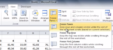
The first thing you’ll do is select the cell that’s in the first column and row that you don’t want to be frozen. Next, go to the View tab and click Freeze Panes. A drop down menu will appear. From here, click on the first option, Freeze Panes.

This will freeze multiple rows and columns in place, which means that they’ll stay in place and visible when you scroll. With your selected rows and columns now frozen, test this out by scrolling sideways, up, and down on your spreadsheet.

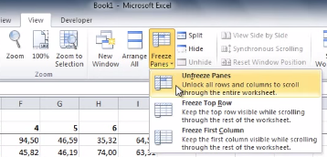
When you’re ready to unfreeze your rows and columns, simply select any row or column and then go to the View tab. Now go to Freeze Panes > Unfreeze Panes.

By freezing columns and rows, you’ll find Excel to be easier to navigate. Check back with Heart of Texas Network Consultants’s blog every week for more time-saving tips.